An introduction to optical Machine Learning

Index

• Introduction
• Light Generation and Manipulation
• The Joint Transform Correlator
• Hong-Ou-Mandel Interferometer
• Future of optical ML
• Bibliography

Introduction

Modern deep learning models (like Gemini or ChatGPT) are trained and deployed in giant datacenters with a collective compute power of several gigawatts. This leads to significant challenges in cost and sustainability as these facilities often require large amounts of water for cooling and place stress on local electrical grids and municipal water infrastructure, which where originally dimentioned for much lower power usage.

Deep learning models leverage massive parallelism, using thousands of specialized cores within GPUs (and increasingly in TPUs) to perform many calculations simultaneously. While GPUs are highly optimized for the linear algebra required by AI, they are still limited by classical digital architecture, which requires every possible solution to be calculated explicitly. In contrast, Quantum Computing can be thought as the “true parallelism of the universe” by using qubits in superposition, these systems can explore vast solution spaces exponentially faster than classical bits. Quantum Computers, by nature, are parallel, they have an infinite number of “cores”. However, this potential efficiency is currently offset by the extreme cooling required to maintain stability and the high error rates (noise) inherent in modern quantum hardware. Another way of achieving parallelism is using light, specifically in optoeletronic computing, where we leverage the characteristics of light (phase, amplitude, wavelength, polarization, etc…) to perform calculations in parallel. This has the advantage of using superposition and doing it at room temperature with minimal hardware and power requirements. In this post we will be exploring two forms of optoeletronic computing: multiple photon phase-modulation (classical computing) and single-photon phase-modulation (true quantum computing).

Light Generation and Manipulation

We will begin by exploring multiple-photon (coherent state) phase-modulation. In this approach, information is encoded into a classical light beam composed of trillions of photons. By manipulating the phase of this coherent beam — essentially shifting its wave cycle relative to a reference — we can perform complex mathematical operations, such as matrix multiplication, with the physical process of interference or Fourier Transform (with a lens). You can think of phase modulation as encoding information into the light beam, like putting a stamp on a paper.

To generate this beam, we utilize an infrared laser with an output power of just 10 mW. To put this efficiency into perspective, a standard household coffee maker consumes 1 kW (1,000 Watts)—enough energy to power 100,000 lasers simultaneously. This giant disparity demonstrates the primary advantage of optoelectronic computing: it moves the ‘energy cost’ of AI from the movement of electrons in metal, that dissipates a lot of energy by heating, to the propagation of light, that dissipates a fraction of the energy.

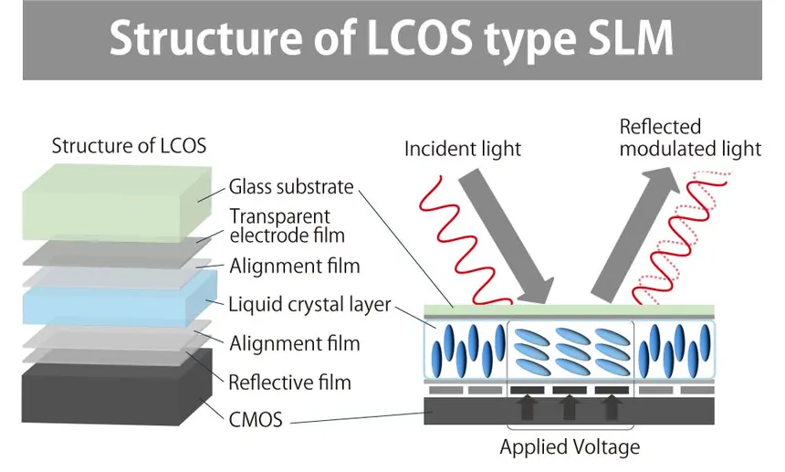
Having discussed how to generate the information medium, we now have to find a way to encode the information (images, text, model weights, etc…) using phase modulation. This is done using a Spacial Light Modulator (SLM), which is a device that electronically controls the spatial distribution of light’s phase. It has multiple layers but is essentialy composed by a liquid crystal layer that, when an electric field is applied, the liquid crystal molecules physically reorient, changing the refractive index of that specific pixel. As light passes through or reflects off this layer, its speed is slightly altered, effectively “shifting” its phase. There are multiple types of SLMs, but the most common are the LCOS (Liquid Crystal on Silicon) SLMs. This alows us to modify the wave front in a grid by up to $2\pi$ (full wave cycle), with a resolution of 1024 levels (10-bit) (depending on the model).

Structure of a reflective phase-only LCOS-SLM. Image taken from Santec's blog post on SLMs.

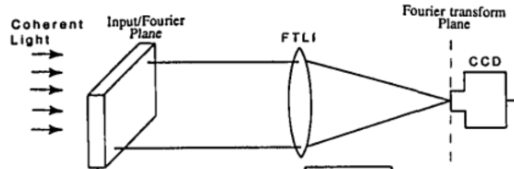
With a way to generate light and modulate it, we can now perform some operations with the light beam. One operation that is complex on a digital computer but is easy to perform with light is the Fourier Transform. The Fourier Transform (FT) has an extremely large number of applications, from signal processing (filtering unwanted frequency components or noise reduction in an image), to solving differential equations, circuits analysis, telecommunications and many more. To perform an Optical FT, we just pass our phase-modulated light through a thin convex lens. By placing a detector, such as a high-speed camera, at the Fourier Plane, exactly one focal length ($f$) away from the lens, the physical diffraction of the light waves automatically performs the transform. In this setup, the lens acts as a natural computer, mapping the spatial information of the input light into its frequency components. To detect the light after performing these operations we use a camera (either CCD or CMOS).

Optical Fourier Transform example setup. The image is encoded into a light beam that is passed through a thin lens, producing the FT. Image taken from Javidi B, Horner JL. Single spatial light modulator joint transform correlator.

The Joint Transform Correlator

Now that we have a way of generating, encoding and perform a FT on the light beam, we can leverage this to perform classification tasks. But how can one do this with such a simple apparatus? How is a single lens doing all of the heavy work?

The Joint Transform Correlator (JTC) is a simple setup that allows for the calculation of the cross-correlation between two signals. The cross-correlation, when evaluated at specific points (correlation peaks), yields the square of the dot product of the two signals. Thus, the JTC calculates a measure of similarity between the two signals, when the signals are similar to each other, the height of the peaks is high, when the signals are different, we see no peaks at all. The matematics of this operation can be a bit tricky, since they involve some FT transforms, so I won’t write it in this blog post, but you can follow the derivation here, in Section III.

Optical Setup of a JTC. The light generated by the laser goes first through a space filtering section followed by an adjust of the polarization and beam expansion. The core section of the JTC is composed of a SLM, a lens and a camera.

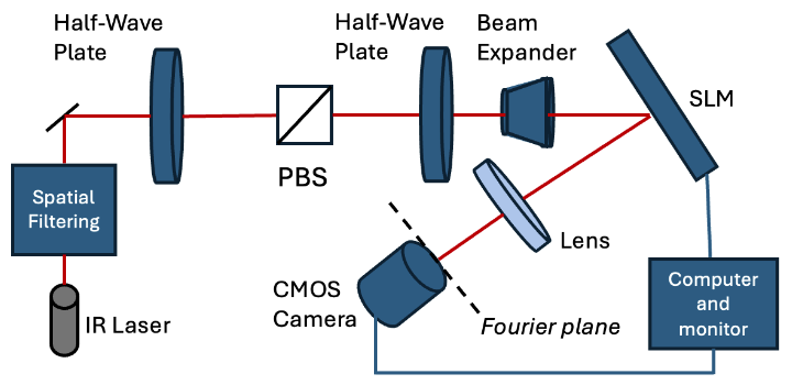
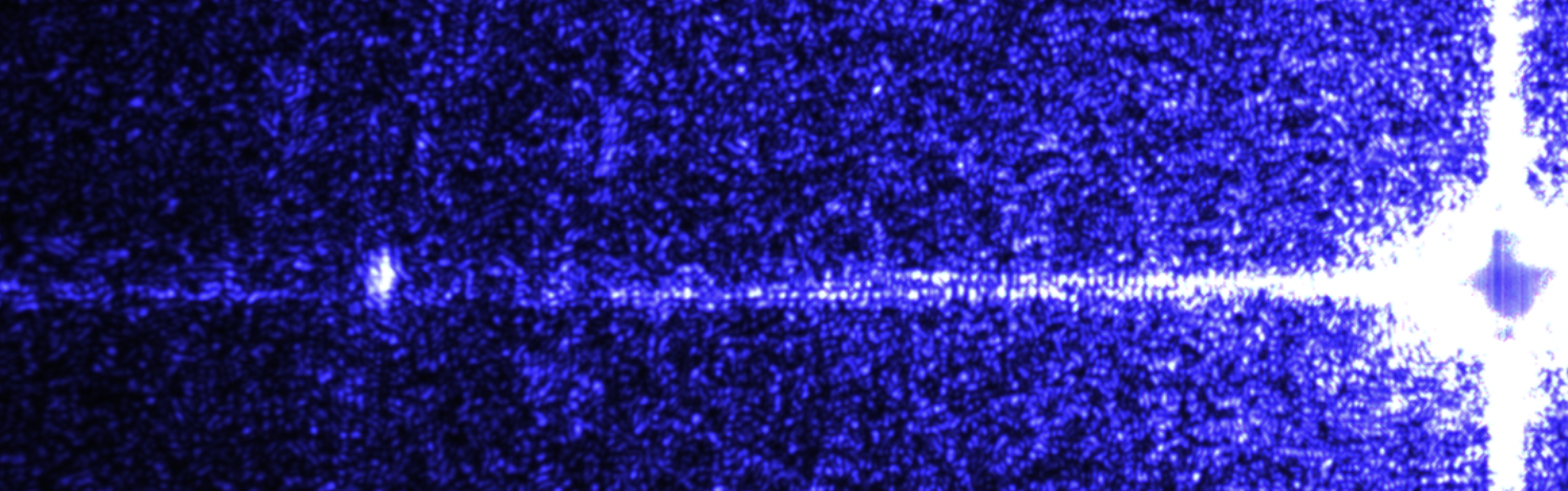
The idea of the JTC is very simple: you place two images side by side on the SLM, pass it through the lens and capture the image with the camera. After that, send the captured image to the SLM again and repeat the process of passing through the lens and capture with a camera. After these two passes, we end up with a so called “correlation plane”, where we see a central (DC) peak, which we can generally ignore, and, if the images are similar to each other, we see cross correlation peaks. Measuring the intensity of these peaks gives us a sense of how similar the images are.

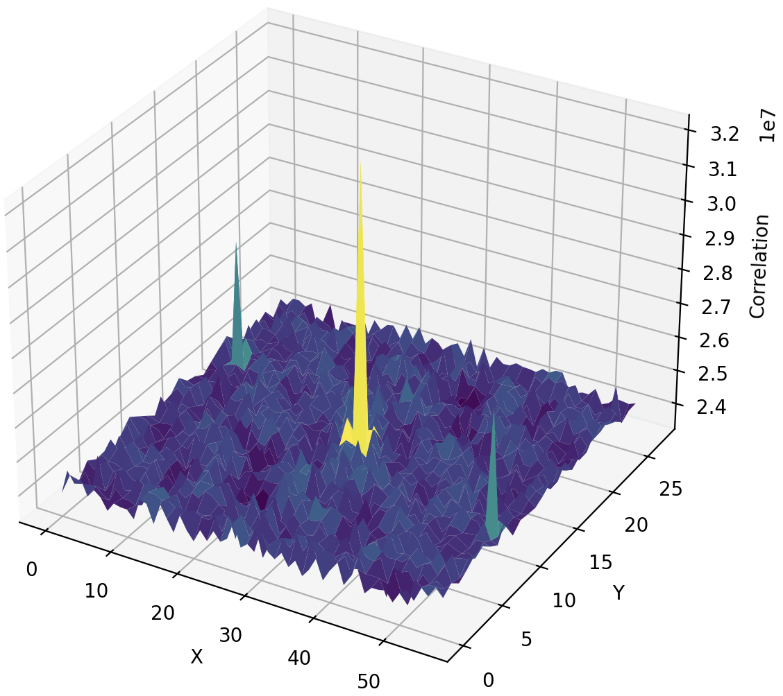
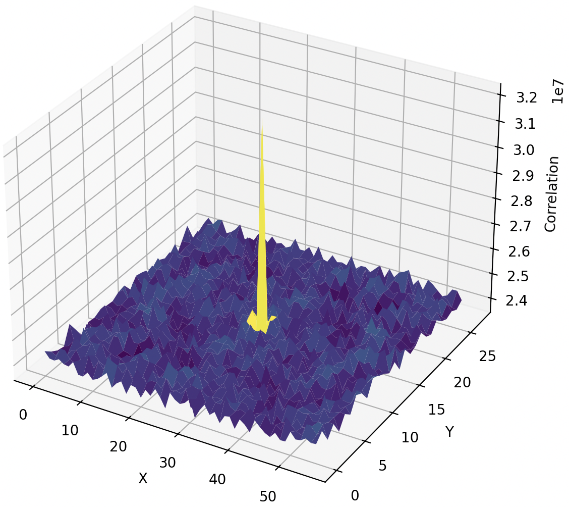
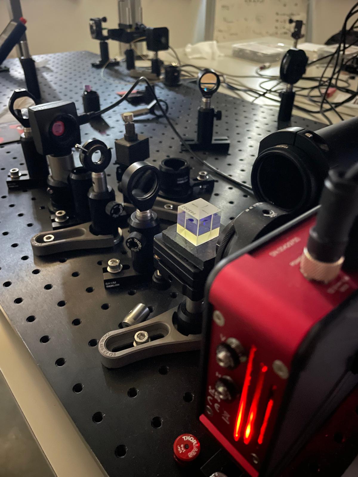
The figures above were created using a computer simulation in Python. Implementing this setup in real life is much more challenging than writing the code. The setup must be carefully aligned, which means aligning every mirror, the SLM, the lens, and the camera. Any slight misalignment leads to distortion in the final correlation plane. There are also some issues like having a specific coating on the lens to prevent unwanted back-reflections, and writing the code to drive and synchronize the camera and the SLM, ensuring the SLM displays the image for the camera to capture multiple times per second. There are always some unexpected issues that arise in the lab; I spent one week just figuring out why there was some distortion of the image after passing through the lens, only to find that it was a form of spherical aberration due to the lens being relatively small for the size of the light beam. Overall, it was very fun and interesting to learn to bridge the gap between the theory and the lab implementation.

Picture of the apparatus in real life. The red device is the SLM, and at the end of the arm we see the camera sensor.

Full correlation plane showing the cross-correlation peaks. This indicates that the images are similar.

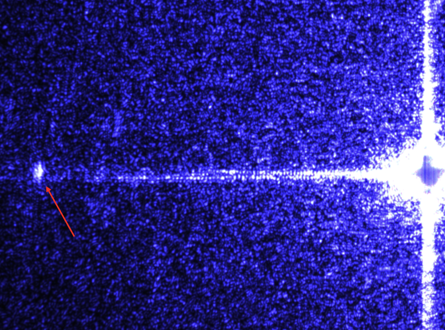
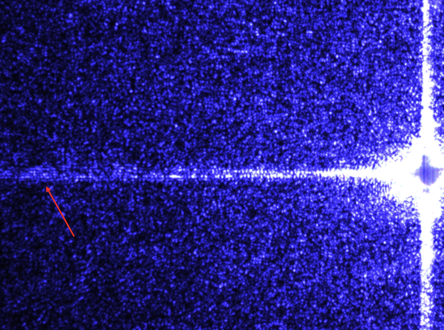
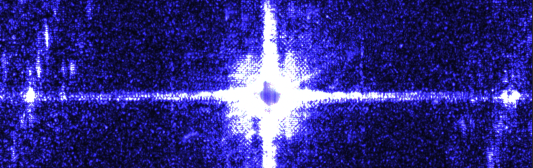
So, the JTC provides a fast, energy-efficient method for calculating the dot product (similarity) between two images, but what actual machine learning algorithms can we implement with it? The most direct application is the nearest-mean classifier. The concept behind this algorithm is straightforward: for each class (in the case of MNIST, this would be each digit from 0 to 9), we calculate the centroid—the average of the pixel values—to generate a representative “average image” for that class. To classify a new input, the algorithm compares it to the reference image of each class and selects the one with the highest similarity. Here, we can exploit the greatest advantage of light: parallelism. Instead of comparing a query image against a single reference image one by one, we can compare the query to all of the reference images simultaneously. This allows us to calculate the similarity of the query to every single class in a single optical operation; we are effectively only limited by the resolution and size of the SLM display. Therefore, we can say that algorithms implemented with a JTC can be inherently multiclass. This characteristic makes the JTC highly suitable for implementing Kernel methods, such as the Support Vector Machine (SVM), since we can essentially calculate the Gram matrix (the dot product between every pair of samples) in parallel, bypassing the serial bottlenecks of digital hardware.

Comparison of the reference digit (average of images in class 1) vs all other digits as query vectors. The algorithm clearly identifies the correct pattern (as a one).

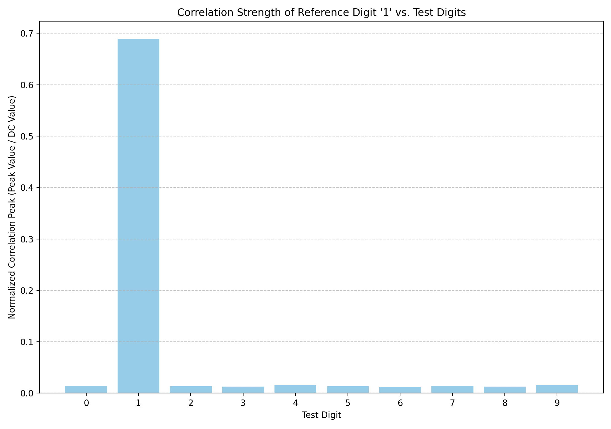
One could also use the JTC non-linearity and embedded convolution mechanism to build a sort of convolutional layer + activation function (non linearity), which could be used in Convolutional Neural Networks (CNNs), but that is content for another whole blog post.

We can also push the JTC beyond classical algorithms, and this is where my own research comes in. The idea of quantum-inspired machine learning is to borrow the mathematical language of quantum mechanics (density matrices, fidelities, quantum distances) while running everything on classical hardware, no single photons or cryogenics required. Instead of comparing images directly, each image is encoded as a density matrix (a pure quantum state), and each class is represented by a quantum centroid: the average of the density matrices of its training samples. Unlike the classical “average image”, the quantum centroid is a mixed state that retains information about the dispersion of the class, information the classical average simply throws away. Classification then becomes: find the centroid closest to the query, according to a quantum distance measure.

The part I find beautiful is that the JTC is naturally suited for this. A density matrix is just a $d \times d$ array of numbers, in other words, an image. So we can display the query’s density matrix and a class centroid side by side on the SLM, exactly like we did with the MNIST digits before, and the correlation peak now reads out the overlap (the quantum fidelity) between the two states. The same lens, the same camera, the same two passes, but now the machine is computing quantum-mechanical overlaps instead of plain image correlations. From this single measurement we can build two quantum distance metrics (the details are in the paper, so I will spare you the formulas), one of which incorporates the purity of each centroid, a single precomputed number per class that tells the classifier how “spread out” that class is.

Does all of this formalism actually help? In my simulations on MNIST it does: the classical nearest-mean classifier reaches an accuracy of 80.37%, while the quantum-inspired version reaches 87.00%, and, somewhat surprisingly, it even beats the exact trace distance (85.83%), the “gold standard” quantum metric that the JTC cannot compute directly. Using two tensor-product copies of each state (the quantum analogue of a polynomial feature expansion), the accuracy climbs to 89.27%, and this is precisely the regime where the exact digital calculation becomes intractable, while the optical measurement stays exactly the same. And this is not just a simulation: the setup shown in the pictures above is the same one running this classifier in the lab, displaying density matrices on the SLM and classifying digits at a rate of a few correlations per second. The current bottleneck is not the optics (the light does its job at, well, the speed of light) but the electronic interface between the computer, the SLM and the camera, which is a very encouraging place for the bottleneck to be.

However, this architecture does not directly translate to modern Neural Networks. While the JTC is highly efficient for specific correlation tasks, it is essentially a fixed, linear operation that lacks the layered depth and trainable weights required for complex deep learning. To achieve that level of abstraction, we need a different approach. We will see next that the Hong-Ou-Mandel (HOM) interferometer can function as a shallow neural network. By moving from the classical regime of interfering trillions of photons to the quantum regime of interfering just two, we can exploit the unique statistics of quantum mechanics to implement the weighted summation and non-linearity of a neuron, effectively creating a quantum perceptron.

Hong-Ou-Mandel Interferometer

What is discussed in this section can be found in this paper and this paper.

With the JTC we were dealing with a light beam with trillions of photons, but in this section we will discuss a single photon, and this is where the true quantum advantage arises. The title of the paper that lead to this is called Quantum optical classifier with superexponential speedup, this means that the setup achieves a superexponential advantage over classical computers by keeping the number of computational operations constant, even as data scales.

Quantum optical neuron implemented by the Hong-Ou-Mandel interferometer. An object is targeted by a single-photon source and classified through the rate of two-photon coincidences at the interferometer output, obtained by placing two photodetectors with no spatial resolution, i.e. without reconstructing the object image. Image taken from "Quantum optical classifier with superexponential speedup" paper.

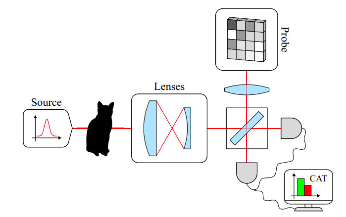
To explain the Hong-Ou-Mandel (HOM) effect, we have to zoom in from the trillions of photons in a laser beam to just two individual photons. In the classical world, if you send two light waves into a beam splitter (a 50:50 mirror), they interfere with each other based on their phase, creating the patterns we saw in the JTC section. But in the quantum world, things get a bit weirder. Imagine we have two independent sources, each firing a single photon at the exact same time towards a beam splitter, one entering from the top, and one from the left. If these two photons are perfectly identical (same color, same polarization, same shape, arriving at the same time), quantum mechanics dictates that they cannot exit separately. They “bunch” together and leave the beam splitter through the same exit port. This means if we place a detector at each output, we will never see them click at the same time. This phenomenon is called the “HOM dip” (because the graph of coincident clicks dips to zero). However, if the photons are distinguishable, say, one is slightly different from the other, they act independently, and the detectors will click together randomly.

Hong-Ou-Mandel coincidence count as a function of the delay of the two photons. When the photons arive at the same time we see a dip in the coincident count, indicating "bunching" behaviour.

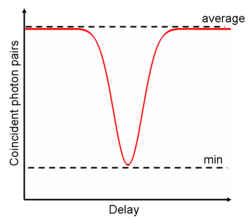
So, how does this help us build a neural network? The clever trick introduced in a recent paper is to use the “shape” of the photon to encode information. Just like we stamped an image onto the laser beam using an SLM in the classical setup, we can impress an input image (like a handwritten ‘7’) onto the spatial profile of the first photon. On the second photon, we encode our “weights” or a reference image (like a perfect template of a ‘7’). Here is the magic: If the input image matches the weights perfectly, the two photons are identical. They bunch together, and our coincidence counter drops to zero. If the input image is very different from the weights, the photons are distinguishable. They exit separately, and we measure a high rate of coincidences. Mathematically, measuring this rate of coincidences gives us the square of the dot product between the input and the weights. This is exactly what a standard artificial neuron does: it multiplies inputs by weights and sums them up. The measurement itself acts as the non-linear activation function (like the ReLU or Sigmoid in digital networks), which is essential for a neural network to learn complex tasks. These weights can be learned by standard gradient descent techniques.

The real power of this approach lies in its scalability. In a classical computer, if you want to compare two high-resolution images, you have to process every single pixel. If the image has 10 million pixels, you need roughly 10 million operations. The computational cost scales linearly ($O(N)$) with the resolution. In the HOM setup, the “comparison” happens through the physical act of interference. Whether the image has 10 pixels or 10 billion pixels, the photons interfere all at once, in a single physical event. We don’t need to calculate the overlap pixel by pixel; we just count the clicks at the detectors. The number of operations is constant ($O(1)$) regardless of the image size. The authors of the paper call this a superexponential speedup. While “exponential” usually implies a massive gain, this is even better: the computational effort effectively flattens out, allowing us to process incredibly detailed data with the same energy and time cost as low-resolution data.

Quantum optical shallow network implemented by a mixed state. One photon collects the input data, e.g. the shape of a object, the other encodes a sequence of hidden parameters, randomly sampled from a set of M different configurations with probabilities acting as output parameters. The input is classified by two bucket detectors that measure the rate of coincidences at the beam splitter output. Image taken from "Quantum optical shallow networks".

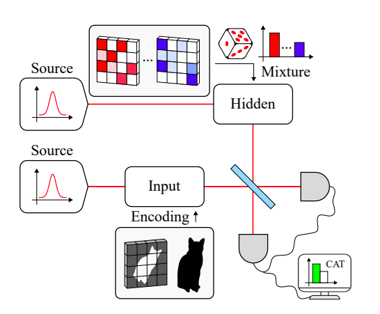
One quantum neuron is good, but to solve more complicated problems (like distinguishing a cat from a dog), we need a Neural Network. A single HOM setup acts as a single neuron, which is a linear classifier as it can only draw a straight line to separate classes. To solve this this, a follow-up study proposed the Quantum Optical Shallow Network. Instead of sending a single “weight” state into the second arm of the interferometer, we send a mixture of states. You can think of this as rapidly switching between different reference patterns or sending a “quantum soup” of multiple learned features. This setup behaves mathematically like a neural network with a hidden layer of multiple neurons. By adjusting the mixture, we can approximate any continuous function, making this system a “universal approximator”. It retains the superexponential advantage: even with multiple virtual neurons and high-resolution inputs, the optical resource cost remains constant for a single classification.

Future of optical ML

Optical computing is not going to replace your GPU next year. Digital electronics have decades of engineering maturity behind them, and the conversion between the electronic and optical domains (cameras, SLMs, drivers) is still the weakest link of every optical processor, both in speed and in precision. But I think the field is at a genuinely exciting point, and there are a few directions that I believe will shape it:

Hybrid pipelines. The most realistic near-term future is not “all-optical AI” but hybrid systems: training stays digital, while the heavy, repetitive linear algebra of inference (dot products, convolutions, Fourier transforms) is offloaded to optics, where it costs almost no energy. The JTC classifier described above is exactly this: the centroids are learned offline on a computer, and the optics only enter at inference time.

Faster and better hardware. The refresh rate of liquid crystal SLMs (around 60 Hz) is the main throughput limit of setups like mine. Ferroelectric SLMs, micro-mirror devices and, above all, photonic integrated circuits — where Mach-Zehnder interferometer meshes perform matrix multiplication on a chip at nanosecond timescales — can raise optical inference rates by many orders of magnitude. The free-space setups of today are the “vacuum tube era” of optical computing; the integrated ones are the transistors.

Smarter encodings and architectures. On the algorithmic side, there is a lot of unexplored territory: encodings that retain norm information without saturating the optical measurements, optical implementations of higher tensor-product states and kernel methods, and architectures beyond the JTC (VanderLugt correlators, diffractive deep neural networks) that trade off complexity, robustness and sensitivity in different ways.

The quantum frontier. And of course, there is the truly quantum path we saw with the HOM interferometer. Single-photon sources and detectors are improving at an impressive pace, and proposals like the quantum optical neuron and the quantum optical shallow network show that meaningful machine learning can be done with just two photons and a beam splitter. If those components become as routine as lasers and cameras are today, the superexponential scaling stops being a theoretical curiosity and starts being an engineering roadmap.

What draws me to this field is that progress requires speaking two languages at once: the abstract language of machine learning and quantum information, and the very concrete language of mirrors, lenses and misaligned optical mounts. As deep learning keeps growing and its energy bill keeps climbing, I believe computing with light will stop being a curiosity and start being a necessity.

If you want the full mathematical details of the JTC and the quantum-inspired classifier, you can find them in my thesis. Thanks for reading, and see you in the next post!

Bibliography

Papers and articles

1. B. J. Shastri et al., “Photonics for artificial intelligence and neuromorphic computing”, Nature Photonics 15, 102–114 (2021).
2. B. Javidi and J. L. Horner, “Single spatial light modulator joint transform correlator”, Applied Optics 28, 1027–1032 (1989).
3. J. Guilherme, “Optical Implementation of Machine Learning Algorithms”, BSc Thesis.
4. L. Huynh et al., “Quantum-inspired machine learning: a survey”, arXiv:2308.11269 (2023).
5. S. Roncallo et al., “Quantum optical classifier with superexponential speedup”, Communications Physics 8 (2025).
6. “Quantum optical shallow networks”, arXiv:2507.21036 (2025).
7. Y. Shen et al., “Deep learning with coherent nanophotonic circuits”, Nature Photonics 11, 441–446 (2017).

Image sources

• Santec, “What is an SLM?” — LCOS-SLM structure diagram.
• Javidi and Horner (ref. 2) — optical Fourier Transform setup.
• Roncallo et al. (ref. 5) — quantum optical neuron diagram.
• “Quantum optical shallow networks” (ref. 6) — quantum optical shallow network diagram.

Wikipedia

• Colossus supercomputer
• Fourier transform
• Charge-coupled device (CCD)
• Image sensor (CMOS)
• Convolutional neural network
• Neural network (machine learning)
• Hong–Ou–Mandel effect
• Universal approximation theorem
• Fidelity of quantum states